Building a Fantasy Football Draft Assistance Algorithm: Part One
Part One – choosing the model, dealing with the data, and generating the model
Context
I’m in a competitive fantasy football league with some friends, with a lot of pride (and a non-insignificant amount of money) on the line. So, when we started the season, I wanted to find any edge I could to help me draft against them (if you’re not familiar with fantasy football, read this first).
Drafting is a core part of fantasy football, and most fantasy football platforms have a recommendation system to assist with drafting players, but I wanted to make my own – as a learning exercise for myself, but mostly as a way to try and beat the recommendations provided by our platform (ESPN). ESPN’s recommendations only use one dataset (their own) for projecting pre-season player projections, and I wanted to see that if I combined several different fantasy fantasy football projection datasets, I could come up with more accurate model for the probability distribution that generates the projected point totals for each player. Hopefully, that model would give me that edge I was looking for. Ultimately, my goal was to make some sort of app that I could run while I was drafting and into which I could feed (1) the player picked and (2) the position in the draft in which that player was picked, and it would return the best possible candidate for every position when it was my turn to pick. I decided to call this app “DAsHA”, which stands for “Draft Assistance Heuristic Algorithm”.
This post is Part One of how I built DAsHA – here, I’ll cover the model that I used to project player performance (and the reason I chose it), how I collected and prepared the various datasets that I needed, and how I generated the model to power the algorithm.
Choosing the Model
Fantasy football point projections are powered by probability distributions – each player has a given probability of scoring your team a given number of points based on the player’s skill, their position, and their week-over-week matchup. Therefore, the model I needed to use had to be one that could estimate a probability density function. One of the classic tools for this type of estimation is a histogram, which works by plotting a curve over a series of buckets that represent different subsets of the range of values in the dataset, and then the data are sorted into the buckets to represent frequency (with the higher buckets representing values that occur more frequently in the dataset). You can fit a Gaussian curve to a histogram to normalize the data, and this gives you a relatively accurate estimation for assessing the probability distribution of a given variable (in our case, fantasy points).
However, one of the drawbacks of a histogram is in its simplicity – since a histogram only uses buckets to represent the data distribution means, the curve that can be fit to a histogram doesn’t actually use all of the sample points: it just uses the buckets. So while modeling my data with a Gaussian histogram seemed like a promising start, I was worried that the curve generated from my histogram wouldn’t be accurate enough to outperform the ESPN projections.
This is where kernel density estimation comes into play. Kernel density estimation is a technique for estimating a probability density function (PDF) that can often outperform histograms, depending on what you want to do. Unlike the histogram, the kernel technique produces smooth estimate of the PDF, uses all sample points’ locations, and more convincingly suggests multimodality. In my case, since I planned on using multiple different buckets of potential scoring projections, I wanted to take advantage of this multimodality, and leverage any potential insights buried therein.
Fortunately, Python has some excellent libraries for implementing Gaussian (Normalized) Kernel Density Estimations (KDEs), and it’s generally a great language for quickly prototyping any sort of data science problem. But before I could do the science, I needed some actual data.
Dealing with the Data
Step 1 - Collecting the data
I wanted a diverse set of projections to improve the accuracy of my KDE, so I collected the projected player performance data from five fantasy football data sources: ESPN, Fantasy Sharks, Fantasy Pros, Fantasy Football Toolbox, and NFL.com. I also used Yahoo!, but their projections, rather than fantasy points, were the the projected fantasy draft positions (this would become important later).
Collecting this data posed a challenge initially, since none of these sources had public APIs (not surprising, but still sad) that I could figure out how to work with, and I didn’t want to write some sort of HTML scraper to import the data into a CSV (nor did I want to reverse-engineer the APIs that they were using to generate the data). Fortunately, though, after a little research (turns out there are a LOT of sports bloggers out there who do stuff like this), I found out that Excel has a native method to import data from the web that just worked out of the box for the above links. Using this speedy approach, I made an Excel spreadsheet for each data source and put them all into the /raw_data directory at the root of my project, like so.
raw_data/
    |-- Yahoo_2020_Draft_Positions.xlsx
    |-- Fantasy_Pros_2020_proj.xlsx
    |-- NFL_2020_proj.xlsx'
    |-- Fantasy_Shark_2020_proj.xlsx
    |-- Sports_Illustrated_2020_proj.xls
    |-- ESPN_2020_proj.xlsx
Step 2 - Preparing the data
Now that I had the data, I could start working on generating the Gaussian KDE. First, I needed to import all the necessary data science libraries that provide user-friendly APIs to help me with that math that I’d need to generate the model. For this project, I used NumPy, pandas, matplotlib, SciPy, and statsmodels.
import numpy as np
import pandas as pd
%matplotlib inline
from scipy import stats
import statsmodels.api as sm
import matplotlib.pyplot as plt
from statsmodels.distributions.mixture_rvs import mixture_rvs
Next, I had to combine everything together into one dataframe. I decided to combine everything together and use the player names from the Yahoo! draft list as the primary index, since my goal for DAsHA is to look up information based on the player nam. What this meant was that my dataframe looked like a 2-dimensional matrix where every player had a list of projected points that corresponded to the various projections that I’d collected. I implemented it like this:
# load Yahoo! draft positions
df = pd.read_excel('./raw_data/Yahoo_2020_Draft_Positions.xlsx')
# strip the names so they can be directly compared to other lists
df['Name'] = df['Name'].str.strip()

# load Fantasy Pros Projections
df_fantasy_pros = pd.read_excel('./raw_data/Fantasy_Pros_2020_proj.xlsx')

# construct temporary data frame to merge relevant info
df_temp = pd.DataFrame()
df_temp['Name'] = df_fantasy_pros['PLAYER'].str.strip()
df_temp['fp_pts'] = df_fantasy_pros['FAN PTS']

# merge df with temporary df
df = pd.merge(df, df_temp, on='Name', how ='outer')

# import NFL projections
df_nfl = pd.read_excel('./raw_data/NFL_2020_proj.xlsx')
df_temp = pd.DataFrame()
df_temp['Name'] = df_nfl['PLAYER'].str.strip()
df_temp['nfl_pts'] = df_nfl['POINTS']

df = pd.merge(df, df_temp, on='Name', how ='outer')

# import ESPN projections
df_espn = pd.read_excel('./raw_data/ESPN_2020_proj.xlsx')
df_temp = pd.DataFrame()
df_temp['Name'] = df_espn['PLAYER'].str.strip()
df_temp['espn_pts'] = df_espn['TOT']

df = pd.merge(df, df_temp, on='Name', how ='outer')

# import Fantasy Shark projections
df_fantasy_shark = pd.read_excel('./raw_data/Fantasy_Shark_2020_proj.xlsx')
df_temp = pd.DataFrame()
df_temp['Name'] = df_fantasy_shark['Name'].str.strip()
df_temp['fs_pts'] = df_fantasy_shark['Fantasy Points']

df = pd.merge(df, df_temp, on='Name', how ='outer')

# import Sports Illustrated projections
df_si = pd.read_excel('./raw_data/Sports_Illustrated_2020_proj.xlsx')
df_temp = pd.DataFrame()
df_temp['Name'] = df_si['PLAYER'].str.strip()
df_temp['si_pts'] = df_si['POINTS']

df = pd.merge(df, df_temp, on='Name', how ='outer')

# Finally, drop the players not available in Yahoo!
df = df.dropna(subset=['Draft Position'])
Running that code gave me the 2-D matrix I needed. Now for the non-parametric fun!
Generating the Gaussian Kernel Density Estimation
Dataframe in hand, I then created a Gaussian KDE for each player using the projected points from each source as the kernels. Each player had 5 sources, so I’d have 5 different kernels per player.
The following code snippet implements the non-parametric estimations for each player. It calculates (1) the median value from the KDE as projected points and (2) the inverse Cumulative Distribution Function (CDF) as an array in kde_icdf so we can generate the non-parametric confidence intervals for DAsHA.
# create an empty column to store point projections for each player
df['pts'] = np.nan

# create an empty column to store the inverse cumulative
# density function (icdf) data for each player's kde estimation
df['kde_icdf'] = [[] for _ in range(len(df))]

# start from index 67 because the first 66 entries in my df
# are contextual cruft and not training data
for j in range(66,len(df)):
    # this block constructs an array of training
    # data for each player of the different fantasy point estimates.
    # This array is used to generate the KDE.
    training_data = []
    training_data.append(df['fp_pts'][j])
    training_data.append(df['nfl_pts'][j])
    training_data.append(df['espn_pts'][j])
    training_data.append(df['fs_pts'][j])
    training_data.append(df['si_pts'][j])
    # clean the training_data for NaN values
    training_data = [x for x in training_data if str(x) != 'nan']
    if len(training_data) == 0:
        training_data = [0]

    # this sets up and runs the non-parametric estimation
    kde = sm.nonparametric.KDEUnivariate(training_data)
    # Estimate the densities
    kde.fit(kernel='gau', bw='silverman', fft=False)

    # This for loop processes to find the median projection
    ci_50 = 0 # initialize median value to zero
    for i in range(0, len(kde.cdf)):
        if kde.cdf[i] < 0.50:
            i+=1
        if kde.cdf[i] >= 0.50:
            ci_50 = kde.support[i]
            break

    # Add data to main dataframe
    df['pts'][j]=ci_50 # add median projection
    df['kde_icdf'][j]=kde.icdf # add icdf for whisker plot construction

# export the dataset to a .csv file
df.to_csv(r'./prepared_data/2020_ffl_df.csv')
The above code takes a while to run, and since I’m an aforementioned python n00b (and because I’d only need to run this once to generate my final dataset), I couldn’t be bothered to speed it up. If you’re a python/data science wizard who has any tips on this, bang my inbox. Something something Cunningham’s law. But anyway, once this code finished running, I had a model for doing KDE estimation!
An applied example of KDE
As the final part of this post, I want include a specific example of how the KDE estimation works for a given draft number to provide context for how DAsHA would ultimately work. In the following code snippet, j represents an arbitrary draft order from which we can generate a Gaussian KDE probability density function for the player corresponding to that draft rank (i.e. it would be represent which pick you’d be making as the fantasy football manager).
j = 125

training_data = []
training_data.append(df['fp_pts'][j])
training_data.append(df['nfl_pts'][j])
training_data.append(df['espn_pts'][j])
training_data.append(df['fs_pts'][j])
training_data.append(df['si_pts'][j])
training_data = [x for x in training_data if str(x) != 'nan']
if len(training_data) == 0:
    training_data = [0]

# this sets up and runs the non-parametric estimation
kde = sm.nonparametric.KDEUnivariate(training_data)
kde.fit(kernel='gau', bw='silverman', fft=False) # Estimate the densities
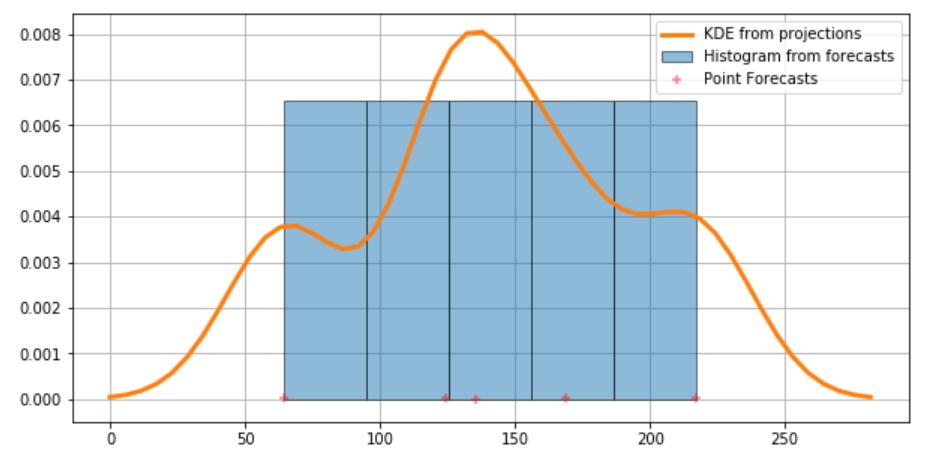
The various point estimates for that player will be indicated by red ‘+’s at the bottom of the graph. The KDE lets us center a normal gaussian distribution (with area = 1/n) for n point estimates) over each of these point estimates. Then, to generate the probability density function, we sum all of these “kernels” together - this summation is the orange line in the graph below.
Finally, the following code snippet generates a histogram from the KDE PDF showing the 1- and 2- standard deviation confidence intervals.
fig = plt.figure(figsize=(10, 5))
ax = fig.add_subplot(111)

# Plot the histrogram
ax.hist(training_data, bins=5, density=True, label='Histogram from forecasts',
        zorder=5, edgecolor='k', alpha=0.5)
# Plot the KDE as fitted using the default arguments
ax.plot(kde.support, kde.density, lw=3,
    label='KDE from projections', zorder=10)

# Plot the samples
ax.scatter(training_data, np.abs(np.random.randn(len(training_data)))/100000,
    marker='+', color='red', zorder=20,
    label='Point Forecasts', alpha=0.5)
ax.legend(loc='best')
ax.grid(True, zorder=-5)
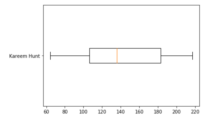
This distribution is then used to generate median point estimations and confidence intervals for each player. For example, this code
box_plot_data=kde.icdf
plt.boxplot(box_plot_data, vert=False, labels=[df['Name'][j]])
plt.show()
generates the following confidence interval for a given player (in this case, Kareem Hunt)
Conclusion and Further Reading
And that’s all for now! I threw a lot of data science concepts out in this post and I don’t want to share too much too quickly. Hopefully, after reading this far you now understand:
- The value of using Gaussian KDEs for projecting fantasy football player performance
- How to collect data to run build this type of model
- How to use popular python libraries to generate a Gaussian KDE from the given data.
In Part Two, we’ll cover how implement this model as a real-time draft assistant tool, and how I used it to out-draft my friends. I look forward to sharing!
Finally, I just wanted to thank my brother, Owen Martin, for code-reviewing my shitty Python. He writes Python all the time and is much better at this than me. Thanks, Bro!